GTMS leverages an open-source software called [https://www.xflr5.tech/xflr5.htm XFLR5] for design and simulation of 2D Airfoils. Download the latest or most recommended version. Your computer will likely give you a warning that the software isn't safe. It is, just hit the more info button to allow it to run.
GTMS leverages an open-source software called [https://www.xflr5.tech/xflr5.htm XFLR5] for design and simulation of 2D Airfoils. Download the latest or most recommended version. Your computer will likely give you a warning that the software isn't safe. It is, just hit the more info button to allow it to run. Follow the steps below to create and analyze a two-dimensional airfoil.
# Open XFLR5. You'll be met with a blank screen
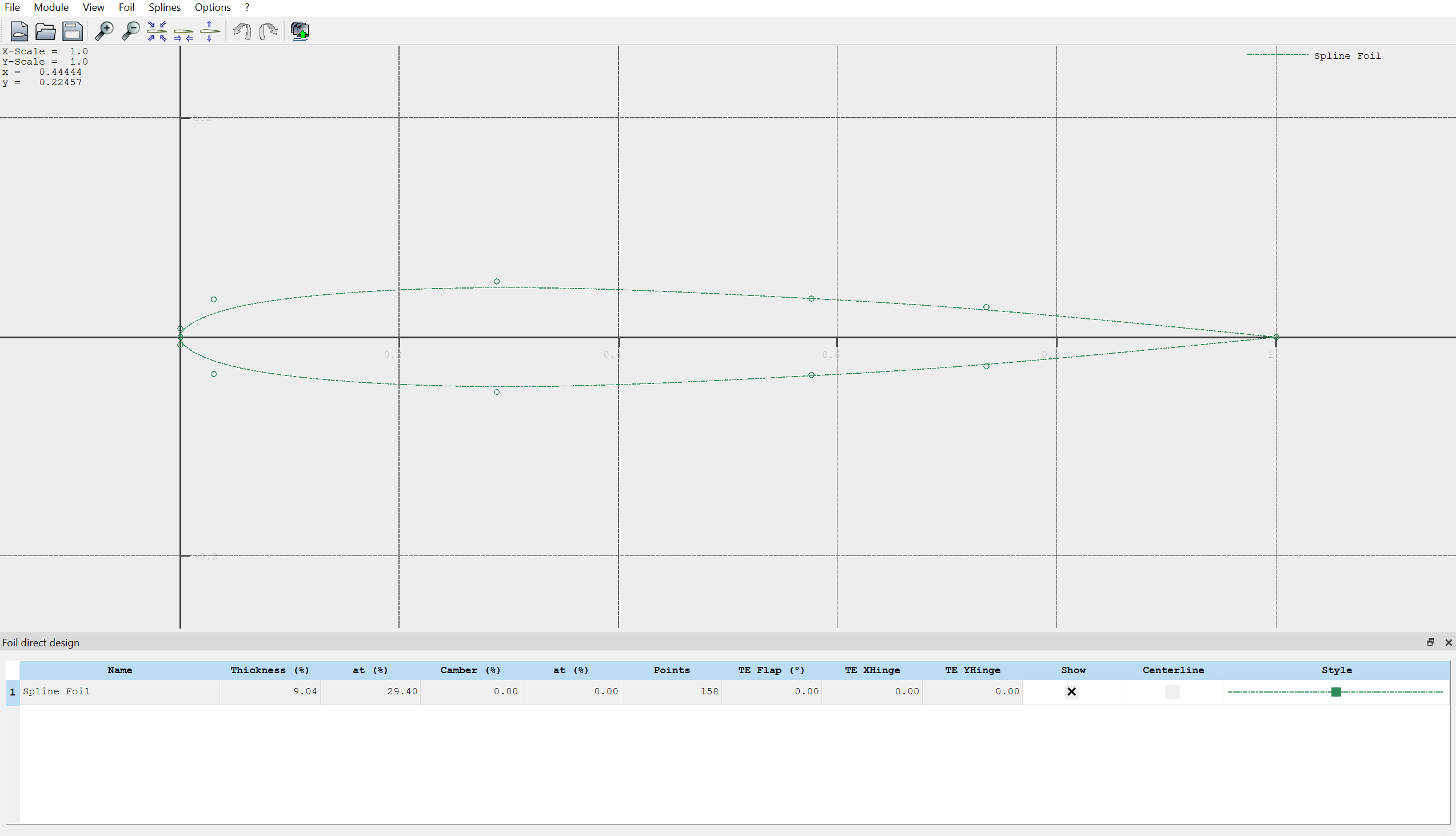
# Navigate to Module -> Direct Foil Design at the top left of the screen. You should see an interface that looks like this:[[File:Xflr5 1.png|center|thumb|600x600px]]
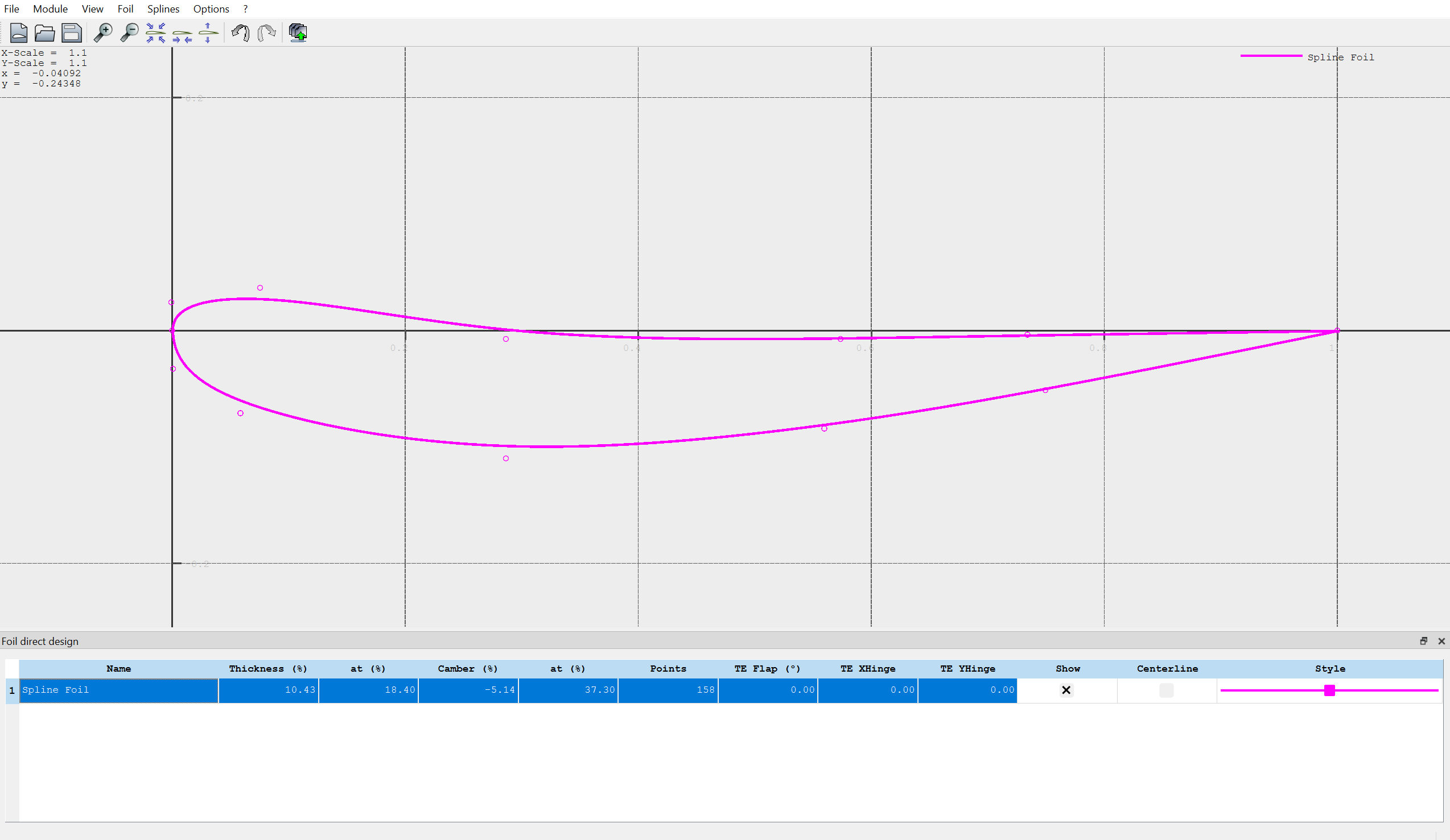
# Click to drag the points you see on screen to make a new spline shape. Yes, it will likely look like a mess your first time making one. You likely barely know what a "good" airfoil is supposed to look like. That's okay! We have resources for that, and this tutorial is just to get familiar with the design procedure. Here's what mine looks like, if you want a reference:[[File:Xflr5 2.png|center|thumb|600x600px|Note that you can change the appearance of your spline by clicking on the "style" tab on the table below your airfoil.]]
# Navigate to Splines -> Store Splines as Foil in the top left. Enter a name with the naming convention (initials)_(type)_(descriptor). Type for our case is sort of ambiguous, but know that "primary", "secondary", and "tertiary" are common designations for the first, second, and third elements of a wing. They are usually abbreviated as "P", "S", and "T". Equally as valid is element 1, element 2, and element 3 which shorten to E1, E2, and E3 respectively. I named the above airfoil "JD_E3_Example".
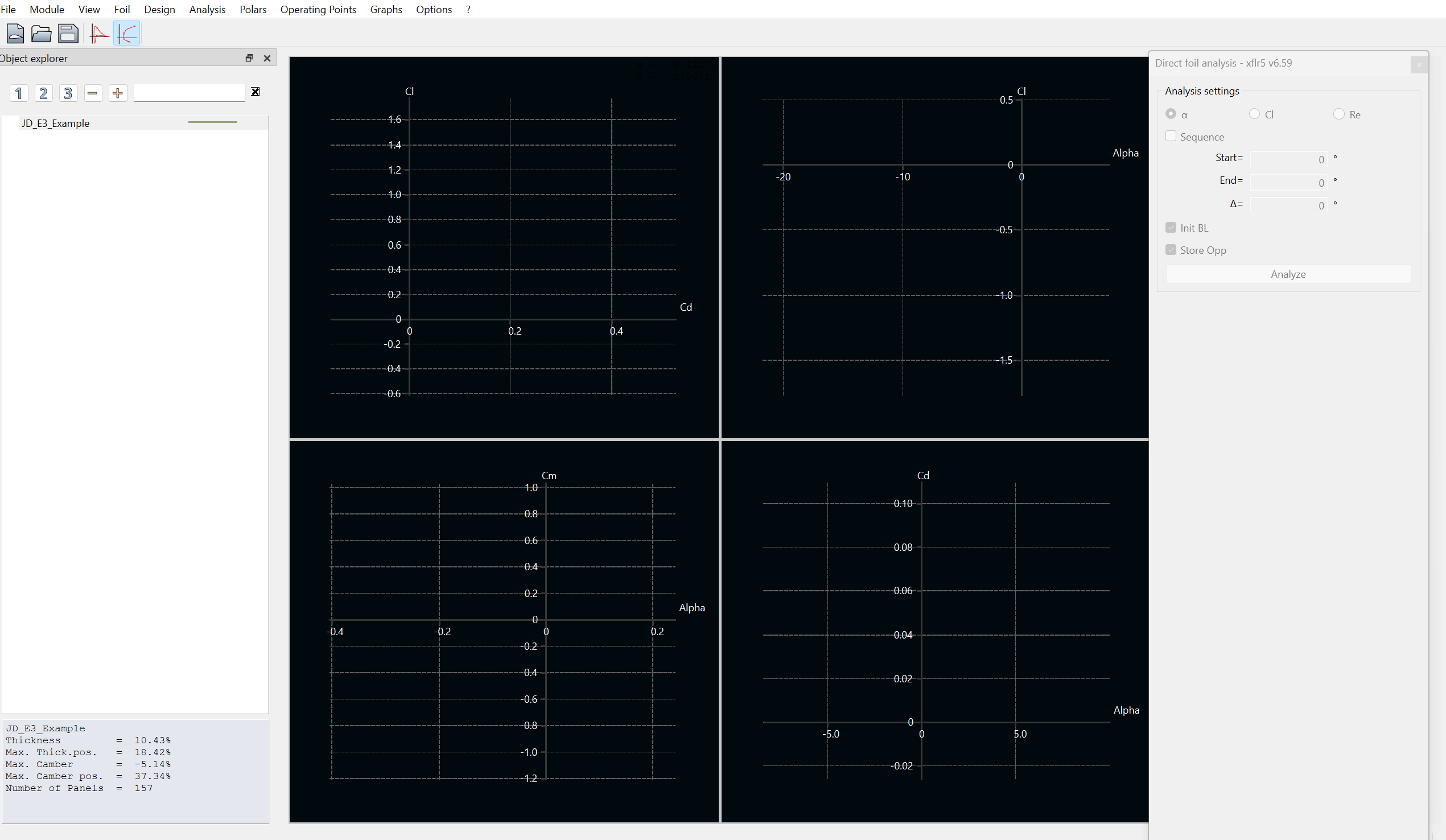
# Navigate to Module -> Direct Foil Analysis. You'll see an interface that looks like this: [[File:Xflr5 3.png|center|thumb|600x600px]]
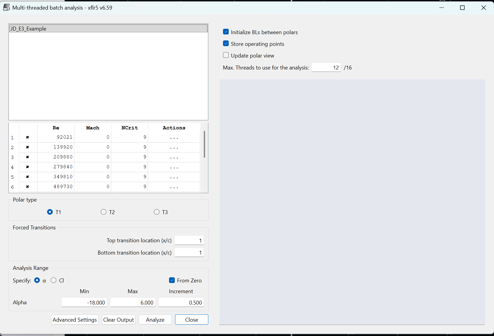
# Navigate to Analysis -> Batch Analysis. It may be a bit confusing for those less experienced from here. Batch analysis allows us to test our airfoil at multiple angles of attack and at multiple [[wikipedia:Reynolds_number|Reynolds Numbers]]. The UI will look like this: [[File:Xflr5 4.png|center|thumb|600x600px]]First, set Min Alpha to -18 and Max Alpha to 6. This defines the range of angles of attack we simulate. Change the increment to 0.500. For Reynolds Numbers, [https://www.omnicalculator.com/physics/reynolds-number calculate] a good range of numbers between 10 and 60 mph at sea level conditions. Assume a characteristic length of 1 m. Use the [https://www.digitaldutch.com/atmoscalc/ 1976 Standard Atmosphere Calculator] to determine dynamic viscosity and density at sea level. One of my personal favorite websites that one, love the little fishes they have at the top. Click the checkbox for Initialize BLs between polars and Store operating points. Change the number of threads such that your computer has four threads available. finally... HIT ANALYZE
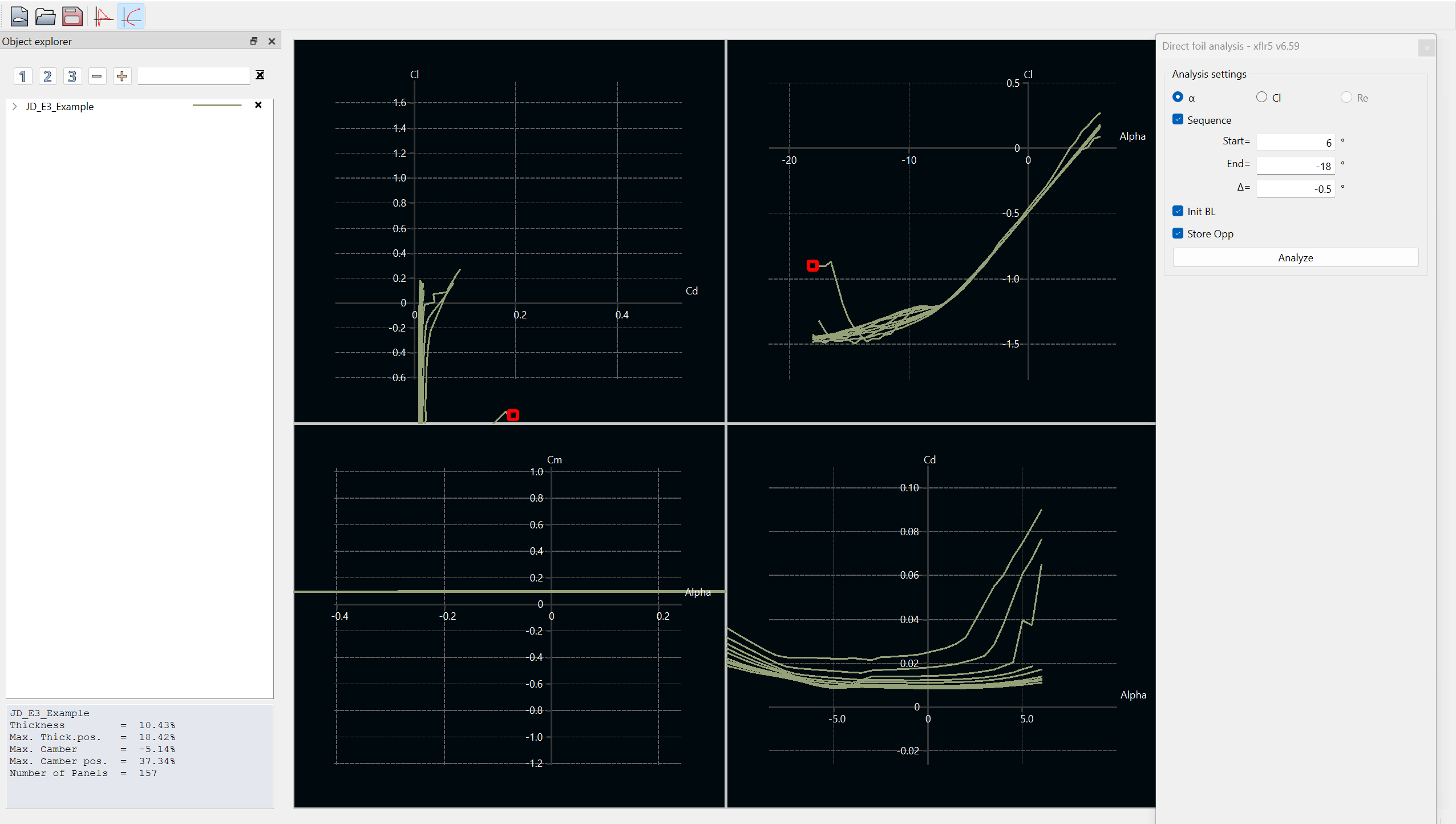
# Exit out of the batch analysis window. You should see the graphs populated with data like so: [[File:Xflr5 5.png|center|thumb|600x600px]]Now what? You just completed your first airfoil simulation! Click and drag the graphs to bring more data into view. Click the dropdown on the left hand side (in the screenshot, the row that says "JD_E3_Example". Clicking the x's will show or hide the data for a specific Reynolds Number of a specific angle of attack point.
==== ''Until I (Jack) finish this tutorial, some food for thought:'' ====
* What is the general trend of Cl versus alpha? Linear? Exponential?
** What is Cl or Cd anyway?
* What is the trend for Cd versus alpha?
* How do these relationships correlate? E.g., what is the relationship between Cl and Cd? Is there a point at which that relationship changes?
* How do the trends differ for different Reynolds Numbers?
* How can I improve airfoil lift? How can I reduce drag?
Revision as of 21:32, 15 October 2025
Airfoils
GTMS leverages an open-source software called XFLR5 for design and simulation of 2D Airfoils. Download the latest or most recommended version. Your computer will likely give you a warning that the software isn't safe. It is, just hit the more info button to allow it to run. Follow the steps below to create and analyze a two-dimensional airfoil.
Open XFLR5. You'll be met with a blank screen
Navigate to Module -> Direct Foil Design at the top left of the screen. You should see an interface that looks like this:
Click to drag the points you see on screen to make a new spline shape. Yes, it will likely look like a mess your first time making one. You likely barely know what a "good" airfoil is supposed to look like. That's okay! We have resources for that, and this tutorial is just to get familiar with the design procedure. Here's what mine looks like, if you want a reference:Note that you can change the appearance of your spline by clicking on the "style" tab on the table below your airfoil.
Navigate to Splines -> Store Splines as Foil in the top left. Enter a name with the naming convention (initials)_(type)_(descriptor). Type for our case is sort of ambiguous, but know that "primary", "secondary", and "tertiary" are common designations for the first, second, and third elements of a wing. They are usually abbreviated as "P", "S", and "T". Equally as valid is element 1, element 2, and element 3 which shorten to E1, E2, and E3 respectively. I named the above airfoil "JD_E3_Example".
Navigate to Module -> Direct Foil Analysis. You'll see an interface that looks like this:
Navigate to Analysis -> Batch Analysis. It may be a bit confusing for those less experienced from here. Batch analysis allows us to test our airfoil at multiple angles of attack and at multiple Reynolds Numbers. The UI will look like this: First, set Min Alpha to -18 and Max Alpha to 6. This defines the range of angles of attack we simulate. Change the increment to 0.500. For Reynolds Numbers, calculate a good range of numbers between 10 and 60 mph at sea level conditions. Assume a characteristic length of 1 m. Use the 1976 Standard Atmosphere Calculator to determine dynamic viscosity and density at sea level. One of my personal favorite websites that one, love the little fishes they have at the top. Click the checkbox for Initialize BLs between polars and Store operating points. Change the number of threads such that your computer has four threads available. finally... HIT ANALYZE
Exit out of the batch analysis window. You should see the graphs populated with data like so: Now what? You just completed your first airfoil simulation! Click and drag the graphs to bring more data into view. Click the dropdown on the left hand side (in the screenshot, the row that says "JD_E3_Example". Clicking the x's will show or hide the data for a specific Reynolds Number of a specific angle of attack point.
Until I (Jack) finish this tutorial, some food for thought:
What is the general trend of Cl versus alpha? Linear? Exponential?
What is Cl or Cd anyway?
What is the trend for Cd versus alpha?
How do these relationships correlate? E.g., what is the relationship between Cl and Cd? Is there a point at which that relationship changes?
How do the trends differ for different Reynolds Numbers?
How can I improve airfoil lift? How can I reduce drag?