Suspension simulation guide: Difference between revisions
JosephBamert (talk | contribs) |
JosephBamert (talk | contribs) |
||
| (One intermediate revision by the same user not shown) | |||
| Line 34: | Line 34: | ||
== Quarter car == | == Quarter car == | ||
[[File:Screenshot 2025-10-27 201111.png|thumb|Quarter car code]] | |||
We will first explore the quarter car code. First all variables are initialized. Unsprung and sprung mass, the damping coefficient, and the spring constant of both the suspension and the tire. | We will first explore the quarter car code. First all variables are initialized. Unsprung and sprung mass, the damping coefficient, and the spring constant of both the suspension and the tire. | ||
| Line 40: | Line 41: | ||
Matrix A is the matrix previous generated in the handcalcs, in this example the state vector is [dot{s}; s; dot{u}; u]). | Matrix A is the matrix previous generated in the handcalcs, in this example the state vector is [dot{s}; s; dot{u}; u]). | ||
Matrix B is the 2nd part of the | Matrix B is the 2nd part of the previous generated matrix- the z component. This represents the road displacement z. | ||
Matrix C | Matrix C is a 4x4 identity matrix. | ||
Matrix D is a 4 row and 1 column matrix full of 0s. | |||
Using the ss (state space) function and inputting the matrices, a state space dynamic system is created. This can then be converted to a transfer function using tf. | |||
Bode and step generate figures demonstrating system dynamics of the quarter car suspension. | |||
Latest revision as of 00:15, 28 October 2025

This is general suspension simulation guide. The force of springs is Fs=-kx. The force of dampers is Fd=-cv. We will be using dot notion to represent derivatives. For example, if x denotes position of a object, ẋ (x-dot) is the velocity of the object, and ẍ (x-double-dot) is the acceleration of the object.
Quarter Car[edit | edit source]
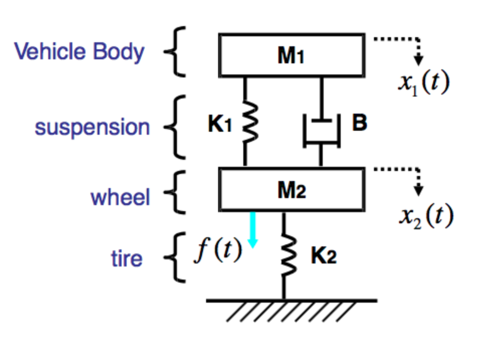
The simplest form to explain the physics of suspension simulation is the quarter car. A quarter car model contains the sprung mass (chassis), coilover spring, the damper (dashpot), unsprung mass, and the tire spring. The tire spring exist because... the tire is a spring and has a stiffness. The sprung mass is supported by the coilover spring and the damper which are connected to the unsprung mass. The unsprung mass is supported by the tire spring.
Coding[edit | edit source]
All MATLAB files can be found on our Github under the vehicle_sim repository.
Toolboxes[edit | edit source]
Go to Home -> Environment -> Add-Ons -> Get Add-Ons. Search for and install the following toolboxes:
- Control System Toolbox
- DSP System Toolbox
- Model Predictive Control Toolbox
- RF Toolbox
- Signal Processing Toolbox
- Communications Toolbox
Important MATLAB functions[edit | edit source]
- Transfer Function (tf): The first input of the transfer function is the numerator and the second is the denominator. Each input is split into coefficients for descending powers of 's'. The output of the tf function is a ratio of polynomials in the Laplace variable 's'. This output can then be analyzed for system properties.
- Example:
- input: num=[2 5] dem=[1 2 3] X = tf(num, dem)
- output:
- Example:
- Step Function (step): computes and plots the step response of a dynamic system. step automatically determines the time steps and duration of the simulation based on the system dynamics. The input is a transfer function and the output is a plot of ___ over time.
- Example
- input: S=step(X)
- output: figure __
- Example
- Bode Function (bode): computers and plots bode frequency response. The input is a transfer function and the output is a plot of phase (deg) and magnitude (dB) over frequency (rad/s)
- Example
- input: B=bode(X)
- output: figure __
- Example
Quarter car[edit | edit source]

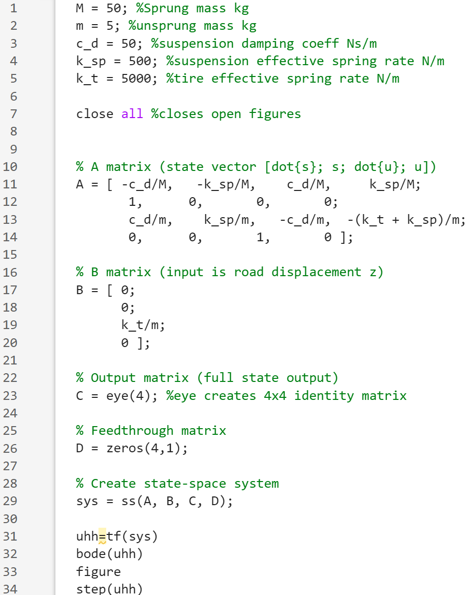
We will first explore the quarter car code. First all variables are initialized. Unsprung and sprung mass, the damping coefficient, and the spring constant of both the suspension and the tire.
"Close all" closes all currently open matlab figures.
Matrix A is the matrix previous generated in the handcalcs, in this example the state vector is [dot{s}; s; dot{u}; u]).
Matrix B is the 2nd part of the previous generated matrix- the z component. This represents the road displacement z.
Matrix C is a 4x4 identity matrix.
Matrix D is a 4 row and 1 column matrix full of 0s.
Using the ss (state space) function and inputting the matrices, a state space dynamic system is created. This can then be converted to a transfer function using tf.
Bode and step generate figures demonstrating system dynamics of the quarter car suspension.